List of Applets for the Chapter Complex Dynamics Chaos

List of Applets for the Chapter
Complex Dynamics Chaos, Fractals, the Mandelbrot Set, and more

This material is based upon work supported by the National Science Foundation under Grant No. 0633125. Any opinions, findings, and conclusions or recommendations expressed in this material are those of the author(s) and do not necessarily reflect the views of the National Science Foundation.

Please contact Rich Stankewitz (rstankewitz@bsu.edu) with any concerns, questions, or suggestions (big or small). The dynamics applets were designed by Rich Stankewitz and Jim Rolf and coded by Jim Rolf.

Due to changes in Java, the applets have been converted to Applications. These do not run in a browser but should be downloaded and run from your local computer. Though these are technically Applications, we retain the word "Applet" when referencing these new tools here and in the linked pages.

Updates to these applets and this webpage will be ongoing. This webpage was last modified on 8-17-11.

Click on the following links to find the applets for this chapter. We hope the applets are intuitive enough to be used without explanation; however, you can find detailed instructions and explanations also by clicking on the following links.

0. ComplexTool Applet - Basic Instructions appear in the text.
1. Real Newton Method Applet
2. Complex Newton Method Applet
3. Real Function Iterator Applet
4. Complex Function Iterator Applet
5. Cubic Polynomial Complex Newton Method Applet
6. Global Complex Iteration Applet for Polynomials
7. Mandelbrot Set Builder Applet
8. Parameter Plane and Julia Set Applet

To see the full text of the book, as well as other book info go to http://www.jimrolf.com/explorationsInComplexVariables.html.

1. Real Newton Method Applet
(currently called Real NewtTool at http://www.jimrolf.com/java/realNewtTool/realNewtTool.html)

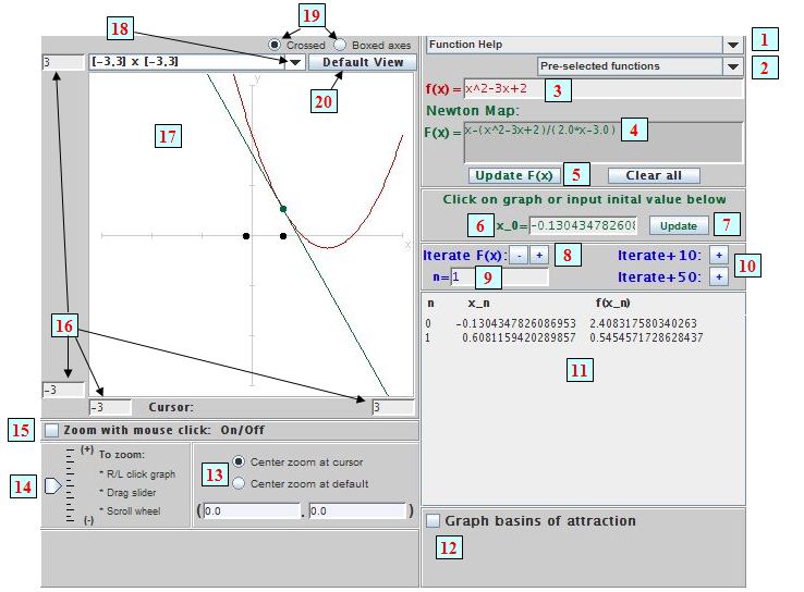
This is an applet to visualize the real-valued Newton's method. This screen shot and text below will guide you through how to use the applet.

Basic Operation: By entering a function f(x) (either by typing it in 3 (with help in 1) or by selecting one from the drop down menu of pre-selected functions 2) and then clicking the Update F(x) button 5, the user will see the graph of f(x) appear in the Viewing window 17 as well as see that the Newton Map F(x) has been calculated 4. By clicking on the graph of f(x), a seed value for Newton's method will be selected and the corresponding tangent line will appear. One can also type in the initial value x_0 directly 6 and then click the Update button 7. One can then iterate the Newton map by clicking on the + button next to Iterate F(x) 8 (or iterate 10 or 50 steps at a time with the corresponding buttons 10). The successive Newton method approximations are then plotted and also displayed in a table 11, along with the corresponding f(x) values. (These values can be copied and pasted into another file in the usual way, if one wishes to.) By typing in a value for n 9 the user can produce the first n Newton approximations x_n. The - button 8 will allow the user to reverse the process, one step at a time.

Zooming on pictures: Zooming on any graph can be done by in a variety of ways.

Depressing the mouse and dragging it across the graph zooms in.
Right/left click on the graph zooms in/out (user will have to first check the Zoom with mouse click on 15).
Scrolling the mouse wheel while the mouse is in the graphing window zooms in/out.
Moving the slider on the zoom panel 14 with a mouse drag or the right/left arrows on the keyboard zooms in/out.

The last three methods of zoom can either be centered at the cursor or at a preset default point 13 (set to (0,0) in the above screen shot). Ctrl+click in viewing window will reset zoom center to the cursor value.

For all zoom methods, the Default View button 20 will return the viewing rectangle to the default setting. Default settings can be changed by selecting one from the drop down menu just above the viewing window 18. The user can also choose their own viewing window parameters by typing in the horizontal and vertical ranges manually 16. This view can then be set as the default by selecting Capture view in the drop down menu 18. Crossed or boxed axes may be selected with the buttons in 19.

Graphing basins of attraction: Do not use the Graph basins of attraction feature until told to do so in the text. To color the basins of attraction check the Graph basins of attraction checkbox and then click on the Graph button that appears. For each seed value in the domain in the current viewing window, the Newton Iterates are computed (up to the number of iterates in the box Max iterations) until the iterates are within Step tolerance of each other, and it is deemed that a root of f(x) has been found. The seed value is then colored according to which root of f(x) it has found, or colored black if no root has been found. This process can be tweaked by the user when new parameters for Max iterations and Step tolerance are entered.

Exporting pictures and Applet Settings:
At the top left of the applet are the following drop down menus:

Export will allow the user to save a png, gif, or jpg picture of the either the whole applet or the viewing window (Graph).
Graph settings will allow the user to adjust various settings such as axes style and color.
Colors will allow the user to adjust the color of the text used in the headings of the various sections of the applet.

2. Complex Newton Method Applet
(currently called Complex NewtTool at http://www.jimrolf.com/java/complexNewtTool/complexNewtTool.html)

This is an applet to visualize the complex-valued Newton's method. The user can operate this applet much like the Real Newton Method Applet discussed above; however, we note a few important changes to keep in mind.

When a function f(z) has been typed in (thus NOT selected by using the Pre-selected f(z) checkbox and corresponding drop down menu), this applet works identically to the Real Newton Method Applet. This process is computationally intensive, and so the applet will sometimes take a few moments to produce a picture when using the Graph basins of attraction feature. However, when using the Pre-defined f(z) checkbox (and corresponding drop down menu) to select f(z), the Graph basins of attraction feature works differently. In this case, since the roots of f(z) are known, the Radius of convergence is used to determine convergence to the roots. Specifically, a seed value is colored when its Newton iterate (up to the number of iterates in the box Max iterations) falls inside a Circle of convergence of one of the roots. This makes this process much faster and so is the preferred method. The Show circles of convergence checkbox make make these circles appear in the graph. The Radius of convergence, i.e., radius of the circles of convergence, can be changed by the user by typing in a new value, and then hitting the Graph button (using the enter key will NOT effect this change). The Plot roots checkbox will make the roots appear. Also, by changing the # color shades value (and then clicking Graph/Update), the basins of attraction will exhibit more shading to help indicate how many iterates are required for a given seed value to enter the circle of convergence. For example, when # color shades is 4, then seed values of the same color and shade will take the same number of iterates mod 4 to enter the circle of convergence.

Thumbnail pictures: Thumbnail pictures at the bottom of the applet record previous pictures which can be restored (along with the corresponding applet parameters) by clicking on them. The most recently created thumbnail has a white border. All thumbnails will be deleted when the Delete thumbnails button is pressed or a new function is selected.

Exporting pictures and Applet Settings:
At the top left of the applet are the following drop down menus:

Export will allow the user to save a png, gif, or jpg picture of the either the whole applet or the viewing window (Graph).
Graph settings will allow the user to adjust various settings such as axes style and color.
Colors will allow the user to adjust the color of the text used in the headings of the various sections of the applet.

3. Real Function Iterator Applet
(currently Real IterTool at http://www.jimrolf.com/java/realIterTool/realIterTool.html)

This is an applet for iterating any real function, and seeing the orbit displayed as a numerical list and as points on a number line. It allows the user to choose up to three seed values at a time and view their orbits.

Basic Operation: By entering a function f(x) either by typing it in (with help from the Function Help drop down menu) or by selecting one from the drop down menu of Pre-selected functions) and then clicking the Graph f(x) button, the user will see the graph of f(x) appear in the Viewing window. By clicking on the graph of f(x), a seed 1 value x_0 will be selected. One can also type in the seed 1 value x_0 directly and then click the Update button. One can then iterate f(x) by clicking on the + button next to Iterate f(x) (or iterate 10 or 50 steps at a time with the corresponding buttons). The successive orbit values are then plotted and also displayed in a table. (These values can be copied and pasted into another file in the usual way, if one wishes to.) By typing in a value for n and clicking on the + button next to Iterate f(x), the user can produce the first n orbit points x_1,..., x_n. The - button will allow the user to reverse the process, one step at a time. Also, by checking the boxes Show seed 2 and Show seed 3, one can choose multiple seed values to be iterated simultaneously.

Zooming on pictures: Zooming on any graph can be done by in a variety of ways.

Depressing the mouse and dragging it across the graph zooms in.
Right/left click on the graph zooms in/out (user will have to first check the Zoom with mouse click on).
Moving the slider on the zoom panel with a mouse drag or the right/left arrows on the keyboard zooms in/out.

The last two methods of zoom can either be centered at the cursor or at a preset default point (set to (0,0) in the above screen shot). Ctrl+click in viewing window will reset zoom center to cursor value.

For all zoom methods, the Default View button will return the viewing rectangle to the default setting. Default settings can be changed by selecting one from the drop down menu just above the viewing window. The user can also choose their own viewing window parameters by typing in the horizontal and vertical ranges manually. This view can then be set as the default by selecting Capture view in the drop down menu. Crossed or boxed axes may be selected with the buttons labeled as such.

Exporting pictures and Applet Settings:
At the top left of the applet are the following drop down menus:

Export will allow the user to save a png, gif, or jpg picture of the either the whole applet or the viewing window (Graph).
Graph settings will allow the user to adjust various settings such as axes style and color.
Colors will allow the user to adjust the color of the text used in the headings of the various sections of the applet.

4. Complex Function Iterator Applet
(currently Complex IterTool at http://www.jimrolf.com/java/complexIterTool/complexIterTool.html)

This is an applet for iterating any complex function, and seeing the orbit displayed as a numerical list and as points plotted in the complex plane. It allows the user to choose up to two seed values at a time and view their orbits. It is very similar in use to the Real Function Iterator Applet and so we explain only the differences here.

This applet allows for either Polar or Euclidean inputs of seed value and independently allows for either Polar or Euclidean computation of functions. Thus in Polar computation mode all seed values will be converted to polar form FOR THE PURPOSE OF COMPUTING THE FUNCTION VALUES and evaluation of the function will be made through the polar form of the map. The Polar computation mode allows only maps of the form z^n.

For example, evaluating the map f(z)=z^2 in Polar computation mode means it will be evaluated as (r, θ) -> (r^2, 2θ). Hence using the seed z_0 = 0.6 + 0.8i in Euclidean seed form and iterating f(z)=z^2 in Polar computation mode will cause the applet to convert z_0 to polar form (r, θ) = (1, arctan (4/3)) and so all computed iterates will be on the unit circle. However, starting with the same seed and iterating f(z)=z^2 in Euclidean computation mode will, due to round off error, cause the orbit to leave the unit circle.

The orbit data is displayed in the same form as the seed value and can be toggled between Euclidean and Polar forms by clicking on the Euclidean seed form and Polar seed form buttons. This applet allows for up to two seed values and includes a checkbox for a thin plot of unit circle to appear (as reference).

Note about computational equivalency: Though mathematically equivalent, the expressions z^2 and z*z are not computationally equivalent. The former is evaluated as exp(2 Log z), where Log z is the principle logarithm, and the latter is evaluated through usual complex multiplication. Thus each will incorporate different rounding errors at times. The end result of this difference is quite evident when iterating the seed 0.6 + 0.8i (on the unit circle) in Euclidean computation mode under each of these maps.

5. Cubic Polynomial Complex Newton Method Applet
(currently Cubic PolyTool at http://www.jimrolf.com/java/cubicPolyTool/cubicPolyTool.html )

This applet allows the user to see the parameter plane and dynamic plane pictures for Newton's method applied to p_ρ(z) = z(z-1)(z-ρ). In the applet, however, the parameter is called a instead of ρ.

Basic Operation: By selecting a value for ρ, either by typing in the value and clicking the Update button or clicking on the (left) Parameter Plane of ρ values window, the basins of attraction for Newton's method are then colored in the (right) Dynamic Plane (for Newton's method) of z values window. The picture is drawn in the same way as in in the Complex Newton Method Applet (when a pre-defined function is selected). Each ρ in the parameter plane is colored according to the root which the free critical point (1+ρ)/3 finds. After clicking in the parameter plane, the ρ value can be moved by using the arrow keys on your keyboard.

In the center of the applet we have the following:

Plot roots of z(z-1)(z-ρ) checkbox which when checked will plot in purple the point 0, 1, ρ, i.e., the roots of p_ρ(z) = z(z-1)(z-ρ).
Show critical orbit checkbox which when checked will plot the critical orbit. Below the ρ value is the Period of the cycle (if any) detected by the critical orbit. The Connect critical orbit points checkbox, when checked, will draw line segments connecting orbit points (to make them easier to see).
Show orbit 1 and Show orbit 2 checkboxes: By clicking in the Dynamic plane viewing window, a seed 1 value z_0 will be selected. One can also type in the seed 1 value directly and then click the Update button. One can then iterate the Newton map F(z) by checking the Iterate orbits checkbox, and then clicking the + button that appears. The successive orbit values are then plotted and also displayed in a table under the Orbits 1 and 2 tab. (These values can be copied and pasted into another file in the usual way, if one wishes to.) By typing in a value for n and clicking on the + button next to Iterate orbits, the user can produce the first n orbit points z_1,..., z_n. The - button will allow the user to reverse the process, one step at a time. Also, by checking the box Show orbit 2, one can choose a second seed value to be iterated simultaneously. After checking the box Show orbit 1 or Show orbit 2, a Connect orbit points checkbox appears which when checked will draw line segments connecting orbit points (to make them easier to see).
Update button will update all pictures and computations based on parameter settings.
Show circles of convergence radius checkbox will show the circles (in the dynamic plane) centered at the roots of p_ρ(z) = z(z-1)(z-ρ) with valid radii of convergence (which were determined via an Additional Exercise in the text) .

Under the Settings tab, the user can adjust the following by entering in a new value and then clicking the Update button

Parameter plane max iterations value is the number points in the critical orbit that must be checked for convergence to a root of p_ρ(z) = z(z-1)(z-ρ) before a ρ value in the parameter plane is colored black.
When a new ρ value is selected by clicking in the Parameter Plane of ρ values a straight line path of k steps is taken between the old ρ value and the new ρ value. At each step, the applet plots the corresponding picture in the dynamic plane. Here k takes on the value listed as the Number of path steps. Also, Delay between path steps is the number of milliseconds the applet pauses before computing the next Dynamic plane picture.
Parameter plane color shades and Dynamic plane color shades determine the number of color shades in each picture.
Root tolerance is a value such that the applet will treat a parameter ρ as 0 when it is within this distance of 0. Similarly, it will treat a parameter ρ as 1 when it is within this distance of 1. For technical reasons, the radii of convergence, and thus the basins of attraction, are calculated differently for such values (since there are only 2 distinct roots of p_ρ(z) = z(z-1)(z-ρ), instead of 3 when ρ is either 0 or 1.
Dynamic plane max iterations value is the number of points in the orbit of each z value that must be checked for convergence to a root of p_ρ(z) = z(z-1)(z-ρ) before that z value in the dynamic plane is colored black.
Dynamic plane min iterations value is the number of iterations made before the convergence condition is checked (default is 0).
Orbit max iterations is the largest number of orbit points that will be plotted for orbit 1, orbit 2, or the critical orbit.
Orbit tolerance is the value used to determine if a periodic point has been found by the critical orbit. If two points on the critical orbit are within this much of each other, then it is deemed that the critical orbit is converging to a cycle.
Parameter plane black/white plot and Dynamic plane black/white plot checkboxes will toggle between a color graph and a black/white graph (without needing to click the Update button).

Zooming on pictures: Zooming on any graph can be done by in a variety of ways.

Depressing the mouse and dragging it across the graph zooms in.
Right/left click on the graph zooms in/out (user will have to first check the Zoom with mouse click on).
Scrolling the mouse wheel while the mouse is in the graphing window zooms in/out.
Moving the slider on the zoom panel with a mouse drag or the right/left arrows on the keyboard zooms in/out.

The last three methods of zoom can either be centered at the cursor or at a preset default point (set to (0,0) in the above screen shot). Ctrl+click in viewing window will reset zoom center to the cursor value.

Thumbnail pictures: Thumbnail pictures at the bottom of the applet record previous pictures which can be restored (along with the corresponding applet parameters) by clicking on them. After creating 30 such thumbnails, the first created thumbnail will be overwritten (thus losing the picture that was previously there). The most recently created thumbnail has a white border (red border if picture is in black/white). The last enlarged thumbnail is surrounded by a yellow border. All thumbnails will be deleted when the Delete thumbnails button is pressed.

Exporting pictures and Applet Settings:
At the top left of the applet are the following drop down menus:

Export will allow the user to save a png, gif, or jpg picture of the either the whole applet or of the individual viewing windows (Parameter plane or Dynamic plane).
Colors will allow the user to adjust the color of the text used in the headings of the various sections of the applet.

6. Global Complex Iteration Applet for Polynomials
(currently called Global Complex Iteration at http://www.jimrolf.com/java/complexPolyIterTool/complexPolyIterTool.html)

When the user to inputs any Polynomial, the applet draws the basin of infinity (with shading that depends on the number of iterates needed to escape, i.e., for an orbit point to have modulus greater than the Dynamic plane escape radius). It will leave seed values black which do not escape after computing the partial orbit up to the value set in Dynamic plane max iterations. It also allows the user to choose up to two seed values at a time and view their orbits.

The applet will actually allow any complex function (not just a polynomial) to be entered in, but the method of drawing the basin of infinity only applies when infinity is an attracting fixed point. Thus the applet will work well for, say, the map z^2+1/z^2, but will not produce accurate results for, say, e^z.

Basic Operation: By typing in a Polynomial f(z) and then clicking the Update button, the user will see the graph of the basin of infinity appear (non-black points) in the viewing window. This process is computationally intensive, and so the applet will sometimes take a few moments to produce a picture. By clicking in the viewing window, a seed 1 value z_0 will be selected. One can also type in the seed 1 value directly and then click the Update button. One can then iterate f(z) by checking the Iterate orbits checkbox, and then clicking the + button that appears. The successive orbit values are then plotted and also displayed in a table under the Orbits 1 and 2 tab. (These values can be copied and pasted into another file in the usual way, if one wishes to.) By typing in a value for n and clicking on the + button next to Iterate orbits, the user can produce the first n orbit points z_1,..., z_n. The - button will allow the user to reverse the process, one step at a time. Also, by checking the box Show orbit 2, one can choose a second seed value to be iterated simultaneously. After checking the box Show orbit 1 or Show orbit 2, a Connect orbit points checkbox appears which when checked will draw line segments connecting orbit points (to make them easier to see). Also, there is a Show dynamic escape radius checkbox that when checked will draw the circle centered at (0, 0) with radius equal to the value set as the Dynamic plane escape radius.

Under the Settings tab, the user can adjust the following by entering in a new value and then clicking the Update button:

Dynamic plane max iterations value is the number points in the orbit of a z value that must be checked for escape before that z value is colored black.
Dynamic plane escape radius determines the escape criterion.
Dynamic plane min iterations value is the number of iterations made before the escape condition is checked (default is 0).
Color sample rate affects how drastically or not the shading colors used in the graph will vary.
Dynamic plane black/white plot checkbox will toggle between a color graph and a black/white graph (without needing to click the Update button).

Zooming on pictures: Zooming on any graph can be done by in a variety of ways.

Depressing the mouse and dragging it across the graph zooms in.
Right/left click on the graph zooms in/out (user will have to first check the Zoom with mouse click on).
Scrolling the mouse wheel while the mouse is in the graphing window zooms in/out.
Moving the slider on the zoom panel with a mouse drag or the right/left arrows on the keyboard zooms in/out.

Thumbnail pictures: Thumbnail pictures at the bottom of the applet record previous pictures which can be restored (along with the corresponding applet parameters) by clicking on them. After creating 22 such thumbnails, the first created thumbnail will be overwritten (thus losing the picture that was previously there). The most recently created thumbnail has a white border (red border if picture is in black/white). The last enlarged thumbnail is surrounded by a yellow border. All thumbnails will be deleted when the Delete thumbnails button is pressed.

Exporting pictures and Applet Settings:
At the top left of the applet are the following drop down menus:

Export will allow the user to save a png, gif, or jpg picture of the either the whole applet or the viewing window (Graph).
Graph settings will allow the user to adjust various settings such as axes style and color.
Colors will allow the user to adjust the color of the text used in the headings of the various sections of the applet.

7. Mandelbrot Set Builder Applet
(at http://www.jimrolf.com/java/mandelbrotBuildTool/mandelbrotBuildTool.html)

By choosing a c value (by clicking in the parameter plane (left) window or inputting it in manually), the point will turn color based on whether or not the critical orbit (computed as far as the value in the Parameter plane maximum iterations input box) escapes for that c value; it will turn red when it escapes and black when it does not. The applet will also plot and list the critical orbit values up to the number entered as the Orbit max iterations. Using the arrow keys on the keyboard after clicking in the Parameter plane window will move the c value by small amounts, updating the critical orbit points as c changes dynamically.

The applet will also allow the user to ``select a square" (by click+drag mouse) in the Parameter Plane and have all the c values in that square colored appropriately which will only be activated after the Color selected square checkbox has been checked (default is unchecked so students do not stumble upon this feature too soon).

Exporting pictures and Applet Settings:
At the top left of the applet are the following drop down menus:

Export will allow the user to save a png, gif, or jpg picture of the either the whole applet or of the individual viewing windows (Parameter plane or Orbit graph).
Graph settings (Parameter or Orbit) will allow the user to adjust various settings such as axes style and color.
Colors will allow the user to adjust the color of the text used in the headings of the various sections of the applet.

8. Parameter Plane and Julia Set Applet
(currently called FractTool at http://www.jimrolf.com/java/fractTool/fractTool.html)

This applet allows the user to see the parameter plane and dynamic plane pictures for several families of functions. The functions one can investigate (via the drop down menu at the top center of the applet) are z^2+c, z^d+c, c*e^z, c*sin(z), c*cos(z), and z^d +c/z^m. It is very similar in use to the Global Complex Iteration Applet for Polynomials and so we explain only the new features here.

Basic Operation: We explain how to use this applet when the family of maps z^2+c is selected, noting that the other families will behave similarly (except for the obvious changes, such as escape criterion). By selecting a value for c, either by typing in the value and clicking the Update button or clicking on the (left) Parameter Plane of c values window, the basin of infinity is then colored in the (right) Dynamic Plane of z values window, with the filled in Julia set colored black. The c value can also be moved around the parameter plane by using the arrow keys on your keyboard.

In the center of the applet we have the following:

Plot fixed points checkbox which when checked will plot in purple the fixed points of the given map z^2+c (only for quadratic maps).
Show critical orbit checkbox which when checked will plot the critical orbit. Below the c value is the Period of the cycle (if any) detected by the critical orbit.
Show orbit 1 and Show orbit 2 checkboxes behave as they do in the Global Complex Iteration Applet for Polynomials.
Update button will update all pictures and computations based on parameter settings.
Iterate orbits checkbox allows the user to generate any/all of the Critical orbit, Orbit 1, or Orbit 2 values. This can be done one step at a time or, by typing in a value for n and hitting the + button to generate the orbit values z_1,..., z_n. The points are displayed in the Dynamic Plane of z values, and the values are listed in the tabs at the bottom. (These values can be copied and pasted into another file in the usual way, if one wishes to.)
Show parameter escape radius and Show dynamic escape radius checkboxes will show the circles (in the parameter plane and dynamic plane, respectively) centered at (0, 0) with the radius prescribed in the Settings tab below.

Under the Settings tab, the user can adjust the following by entering in a new value and then clicking the Update button

Parameter plane max iterations value is the number points in the critical orbit that must be checked for escape before a c value in the parameter plane is colored black.
Parameter plane escape radius determines the escape criterion for the critical orbit when coloring the parameter plane.
When a new c value is selected by clicking in the Parameter Plane of c values a straight line path of k steps is taken between the old c value and the new c value. At each step, the applet plots the corresponding picture in the dynamic plane. Here k takes on the value listed as the Number of path steps. Also, Delay between path steps is the number of milliseconds the applet pauses before computing the next Julia set.
Color sample rate affects how drastically or not the shading colors used in the graphs will vary.
Dynamic plane max iterations value is the number points in the orbit of a z value that must be checked for escape before that z value in the dynamic plane is colored black.
Dynamic plane escape radius determines the escape criterion when coloring the dynamic plane.
Dynamic plane min iterations value is the number of iterations made before the escape condition is checked (default is 0).
Period detection max iterations is the largest number of points in the critical orbit which will be computed when determning the period of a cycle (if any) detected by the critical orbit..
Period detection tolerance is the value used to determine if a periodic point has been found by the critical orbit. If two points on the critical orbit are within this much of each other, then it is deemed that the critical orbit is converging to a cycle.
Parameter plane black/white plot and Dynamic plane black/white plot checkboxes will toggle between a color graph and a black/white graph (without needing to click the Update button).

Thumbnail pictures: Thumbnail pictures at the bottom of the applet record previous pictures which can be restored (along with the corresponding applet parameters) by clicking on them. After creating 30 such thumbnails, the first created thumbnail will be overwritten (thus losing the picture that was previously there). The most recently created thumbnail has a white border (red border if picture is in black/white). The last enlarged thumbnail is surrounded by a yellow border. All thumbnails will be deleted when the Delete thumbnails button is pressed or a new family of maps is selected.

Exporting pictures and Applet Settings:
At the top left of the applet are the following drop down menus:

Export will allow the user to save a png, gif, or jpg picture of the either the whole applet or of the individual viewing windows (Parameter plane or Dynamic plane).
Colors will allow the user to adjust the color of the text used in the headings of the various sections of the applet.

Note: The family of functions z^w+c = exp(w Log z) + c, where Log z is the principle logarithm for complex constants w and c has been added. The "Julia" set pictures in the dynamic plane represent the split between points with bounded orbit and points with unbounded orbit. The parameter plane represents the split between those c values for which the origin escapes and those for which it does not. However, these maps are not in general analytic and so one must apply the general theory with great caution.